Fed policy is more complex in this post-QE world
The way we think about monetary policy has changed with the adoption of quantitative easing (QE) prompted by the global financial crisis: It has moved from being a one-dimensional problem of only setting the policy rate (PR) to a two-dimensional problem of jointly determining the PR and QE.
Central banks — in particular those that undertook QE — are now moving along a path toward policy normalization. This will come at different speeds, and in fits and starts, as conditions evolve. But the question of whether QE will be a part of the policy landscape once normalization is achieved remains topical.
Will central banks conduct monetary policy with not one, but two instruments — PR and QE? What does permanent QE mean for policy communications, the predictive power of the yield curve and overall risk-taking in the financial sector?
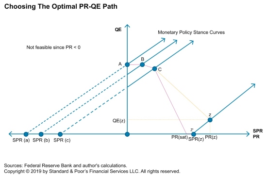
We would argue that, in the case of the Fed, monetary policy is already a two-dimensional exercise and has been since the PR lifted off of zero in late 2015 (A to B in the chart). From that time onward, both the PR and QE were positive. This had never happened before.
The fact that monetary policy is now in the positive quadrant of PR-QE space, and not “on the corners” means choices need to be made about the combination of the PR and QE. This represents a new type of policy optimization problem.
How should central banks normalizing their policy stance to formulate and execute this PR versus QE choice? Like any optimization problem, we need a constraint and an objective.
Note that any combination of a PR and a level of QE translates into a shadow policy rate (SPR). Unlike the PR, which has a lower bound of zero, the SPR can be negative. Corresponding to every SPR, there is an upward sloping curve (or line) in PR-QE space, along which the monetary policy stance (MPS) is constant.
Why does the constant MPS line slope upward? Because QE, by lowering medium-term bond yields, eases monetary conditions while raising the PR tightens them. Importantly, the central bank can “buy” a higher PR by undertaking more QE while keeping the MPS constant.
In terms of its constraint, the central bank, once it has chosen its policy stance, can pick any PR-QE combination along an upward sloping MPS curve in order to achieve its objective.
To determine which point along the MPS curve a central bank will choose, we need preferences. Let’s keep this simple. First, assume that more PR is good; this is especially true when the PR is close to zero and the central bank needs space to maneuver, but less so as PR rises.
Second, assume that more QE is bad since bond purchases by the central bank “artificially” lower yields and therefore push up asset prices and force investors down the credit curve, increasing systemic risk. This distortion starts modestly at low QE levels, but gets worse as QE rises.

How does the central bank solve its problem? It first chooses an MPS corresponding to a SPR that will achieve its objective. It then optimizes according to the following rule: The trade-off in benefits between PR and QE should be equal to the slope of the MPS curve.
Some intuition: Starting at a low PR-QE and moving up an MPS curve, the initial gains from increasing PR are relatively high and the cost of increasing QE is relatively low. Net gains are high. But as we continue to increase PR and QE, these net gains decline as PR space is more sufficient and QE is more distortive.
At some point, the net gain from higher PR and QE matches the slope of the MPS curve. Going any further is not optimal. For each MPS curve there is a unique PR-QE combination that solves the central bank’s maximization problem.
Finally, the big questions to consider: Where does the optimal PR-QE combination end up? Is QE positive or not? Is monetary policy one- or two-dimensional? As the central bank normalizes policy, by raising SPR with corresponding rightward shifts in the MPS, we can trace out the path of optimal PR-QE combinations. These are points A, B and C in the chart.
The terminal (neutral) stance is denoted by MPS(z) and two possible PR-QE paths are shown. For the green path the central bank ends up at Z with a positive level of QE, with PR(z) greater than SPR(z). It has bought some extra policy rate space by engaging in QE(z).
In contrast, for the red path, the central bank has enough policy rate ammunition (it is satiated) and ends up at Z’. On this path, for any policy rate above PR(sat) there is no QE and PR equals SPR. We are back to a one-dimensional world. The difference between the two paths lies in the central bank’s preferences.

We explore the model more formally as well as related permanent QE issues in the full paper.
Paul Gruenwald is the chief global economist at S&P Global Ratings.
Copyright 2024 Nexstar Media Inc. All rights reserved. This material may not be published, broadcast, rewritten, or redistributed..


